Note: for details on how any of the plots were made in this blog post, see our paper.

The mystery of generalization

The power of neural networks lies in their ability to fit almost any kind of data (their expressiveness), and in their ability to generalize to new data sampled from the same underlying distribution. The expressiveness of neural networks comes from the fact that they have many parameters that can be optimized to fit the training set, which usually has fewer data points than the number of model parameters. Under such overparametrized conditions, it is possible for networks to perfectly fit the training data while performing poorly on the unseen test data. Yet, peculiarly, neural networks tend to generalize well even when no regularizers are in place during training.

One common explanation is that neural net optimizers are inherently biased toward good minima. The stochasticity of the optimizer (Keskar et al. 2016), and the optimizer’s update rule (Bello et al. 2017) both cause percent-level improvements in generalization, but these changes are small, and the generalization is still relatively high (with generalization gap not usually exceeding 10%) for any choice of optimizer.

Yet, overparametrization means we shouldn’t expect any generalizability. On CIFAR-10, simply fitting the training set perfectly should not lead to around 90% test accuracy as it usually does, but rather to accuracies approaching 10% (random-chance). Yet we never see any accuracies even remotely that bad, which means that the structure of neural networks lend some implicit regularization, or inductive bias, or “prior” to the learner to help it generalize. To what prior, then, does the credit belong?

The wide margin prior

A traditional regularization (or prior) used in support vector machines (SVM) is to encourage wide margin decision boundaries. This took the form of a hinge loss on a linear classifier over SVM kernels. A classifier whose decision boundary is far from any training point is more likely to classify new data correctly.

In neural nets, the wide margin condition is closely associated with the flatness of the neural loss surface around the minimizer. To see this, consider that a small perturbation to the parameter vector causes a small change in the shape/position of the decision boundary. Under the wide margin condition, small changes in the boundary should not lead to much misclassification. If all possible small perturbations of the parameter vector lead to low misclassification, then the loss surface around that minimizer does not rise much in any direction, and is thus considered “flat”.

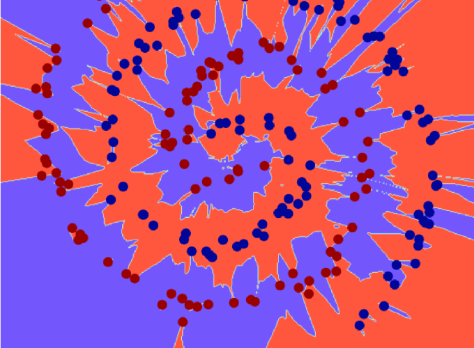
We visualize this with a toy dataset in the figure below. The left is a wide margin model and the right is a narrow margin model. Both perfectly classify the training data (denoted as red/blue dots), but the narrow margin model’s decision boundary barely wraps the data on little ‘peninsulas’ or ‘islands’ such that each data point is extremely close to the boundary. The generalization of the wide margin model is far better than that of the narrow margin model (100% test accuracy vs 7%). The loss surface in parameter space corresponding to each model are plotted in the bottom row, showing that the wide margin model has a much flatter and wider minimizer than the narrow margin model.

The two animations below show what happens when the parameter vector is perturbed. The loss surface (xent), training accuracy (acc), loss surface curvature (curv) are plotted as well to show the correlation between loss surface flatness and margin width.

Since its decision boundary is far from the data points, perturbations do not cause the wide margin model to misclassify until the perturbation is quite large. This is manifest in a very flat minimizer (see xent curve)

Meanwhile the narrow margin model immediately loses performance when the parameters are slightly perturbed, since its decision boundary is so close to each of the data points. The loss goes up much faster around the minimizer.

Both of the above models have the exact same architecture (6-layer fully connected network). They simply occupy different points in the same high dimensional parameter space.

Flat minima, wide margin, and generalization: a closer look

So flat minima lead to wide margin which leads to good generalization—great. But what prior or regularizer implicitly biases neural network parameters toward flat minima? We will see that the process of naturally training a network without explicit regularizers is already intrinsically biased toward flat minima based on a simple volumetric argument.

In search of bad minima

Though we do not naturally find them, suppose that a configuration of parameters exists with near-random generalization performance. We can train explicitly find bad generalizers by penalizing good generalization, aka correct predictions on unseen data drawn from the true distribution, via the following loss function.

$$ L = \frac{1-\beta}{\left|\mathcal{D}_{train}\right|} \sum_{x,y\in\mathcal{D_{train}}} y\log p_{\theta}(x) + \frac{\beta}{\left|\mathcal{D}_{true}\right|}\sum_{x,y\in\mathcal{D_{true}}}y\log[1-p_{\theta}(x)] $$

The first term is the cross entropy loss on the training set $\mathcal{D}_{train}$, to ensure that we still get low loss on the training set. The second term is the cross entropy on data sampled from the “true” distribution $\mathcal{D}_{true}$. Typically the true distribution is not known, but in our toy example of the swiss roll, it is defined by us. For images, this distribution can be approximated by a GAN. In the second term—the softmax probability is reversed (i.e. we substitute $p_\theta(x)$ with $1-p_\theta(x)$) This has the effect of encouraging the network to decrease (rather than increase) its prediction probability of the true class, akin to poison attacks which flip the training labels in order to disable a trained model. If both of these terms are minimized, the network will learn a parameter configuration $\theta$ that performs well on the training set, but poorly on all other data drawn from that distribution. $\beta$, or the poison factor, is the fraction of each minibatch consisting of poison examples.

Good minima are exponentially easier to find

We can modulate the poison factor to control the amount of generalization that a trained network achieves. In the figure below we show that the train/test gap (aka generalization gap) is correlated with the poison factor. To show that our results extend beyond a simple toy dataset, we also perform the same experiments on the Street View House Numbers (SVHN) dataset.

Modulating the poison factor also allows us to visualize the margin of the decision boundary as the network goes from a good to bad minimizer.

To characterize the flatness, we define the basin to be the set of points in the neighborhood the minimizer having a loss value below a certain cutoff value. We plot the basin along multiple random directions in the high dimensional loss surface in the figure below. Note that the basin radius $r(\phi)$ along a direction $\phi$ is defined as the distance from the minimizer to the cutoff point along that direction.

The probability of colliding with a region during a stochastic search does not scale with the width of this basin, but with its volume. Network parameters live in very high dimensional spaces where small differences in the basin radius translate to exponentially large disparities in the basin volume. Therefore, good, large-volume minima are exponentially easier to find than bad, small-volume minima. We characterize the volume of our found minima through simple Monte-Carlo estimation. The figure below shows a scatter plot between (log) volume and generalization gap for various cutoffs.

For SVHN, the basins surrounding good minima have a volume at least 10,000 orders of magnitude larger than that of bad minima (!!), rendering it impossible to stumble upon bad minima in practice.

Conclusion

The reasons for why non-regularized, overparametrized neural networks tend to generalize has attracted much attention in the research community, but there have not been many which have focused on an intuitive explanation. Through empirical evidence and visualizations, we show that naturally trained neural networks have an intrinsic wide margin regularizer (prior) which enable them to generalize the same way that SVM’s do with their explicit wide margin criteria. We argue that flat minima lead to wide margin which in turn leads to good generalization, and that such flat minima are exponentially easier to find than sharp minima due to their exponentially larger volume in high dimensional spaces.

Acknowledgement: A shoutout to CometML, which was my go-to for debugging, diagnosing, versioning, and storing all artifacts generated in this research. Comet not only has a great UI, it also stored all the logs, data, and plots generated in this project, so I could focus on research rather than searching for logs or managing my file system.